Mall-Customers-Segmentation
This project uses Python to analyze a customer dataset from a mall.
Dataset
The dataset includes the following columns:
- CustomerID: Unique identifier for each customer
- Gender: Male or Female
- Age: Age of the customer
- Annual Income (k$): Annual income in thousands of dollars
- Spending Score (1-100): Score assigned by the mall based on customer behavior
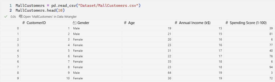
Loading and reading the dataset
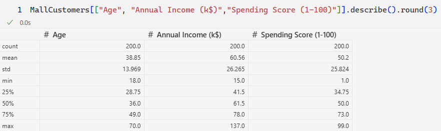
Basic statistics
Distribution Analysis of the customer data
| Metric | Key Takeaway |
|---|---|
| Age | The customer base is dominated by Young Adults (25-40), with a secondary, smaller segment of middle-aged customers (45-55). |
| Annual Income (k$) | The majority of customers fall into a mid-income bracket ($50k to $80k). |
| Spending Score (1-100) | Most customers exhibit an average spending pattern, clustering between 40 and 70. |
The data indicates a customer base primarily composed of mid-income young adults with average spending habits. This pattern suggests the need for customer segmentation to identify outliers and higher-value groups.
Gender Based Distribution
 |
 |
 |
 |
Gender-Based Analysis Summary
The comparative analysis by gender highlights key differences across the customer base.
| Visualization | Key Finding | Interpretation |
|---|---|---|
| Gender Pie Chart | The customer base is majority Female (56%) compared to Male (44%). | Any communication or marketing effort will naturally reach more female customers. |
| Age by Gender (KDE) | Female customers are significantly younger, with the peak density around age 30. Male customers have a broader, flatter age distribution. | Young adult females (ages 25-40) represent a highly concentrated segment. |
| Income by Gender (KDE) | Annual Income distributions are nearly identical for both genders, centering in the mid-income range ($60k - $70k). | Income level is not a differentiator between the male and female segments. |
| Spending Score by Gender (KDE) | Female customers are tightly clustered in the average spending range (45-60). Male customers have a higher proportion in the low-spending range (0-40). | Female customers are more consistent, reliable spenders, whereas male customers are more likely to be low-volume purchasers. |
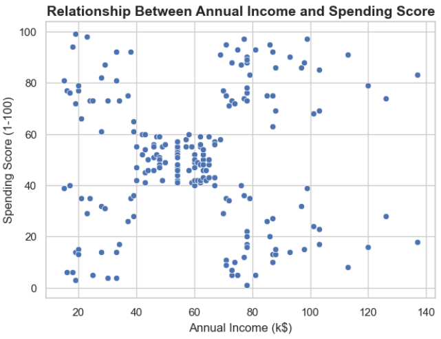
Relationship Between Annual Income and Spending Score
Segmentation Analysis: Income vs. Spending
This scatter plot is the foundation for customer segmentation, revealing five distinct clusters based on the relationship between Annual Income and Spending Score. This structure strongly suggests that K-Means Clustering will be an effective modeling technique.
| Cluster | Income Range (k$) | Spending Score (1-100) | Segmentation Profile | Business Strategy |
|---|---|---|---|---|
| High-Value VIP | High ($70+) | High ($75-100) | Wealthy and high-spending. | Retention & Loyalty: Focus on exclusive services and personalized offers. |
| Average Market | Medium ($40-70) | Medium ($40-60) | The largest and most typical customer group. | Volume & Cross-Sell: Standard promotions and broad marketing campaigns. |
| High Potential | High ($70+) | Low ($0-40) | High income but currently under-spending. | Activation: Investigate reasons for low spending and target with product recommendations. |
| Budget Spender | Low ($15-40) | Low ($0-40) | Low income and low spending. | Cost Sensitivity: Focus on value deals, discounts, and clear promotions. |
| Impulsive Spender | Low ($15-40) | High ($70-100) | Low income but high spending. | Risk Management: Focus on immediate sales volume, but monitor for potential churn/risk. |
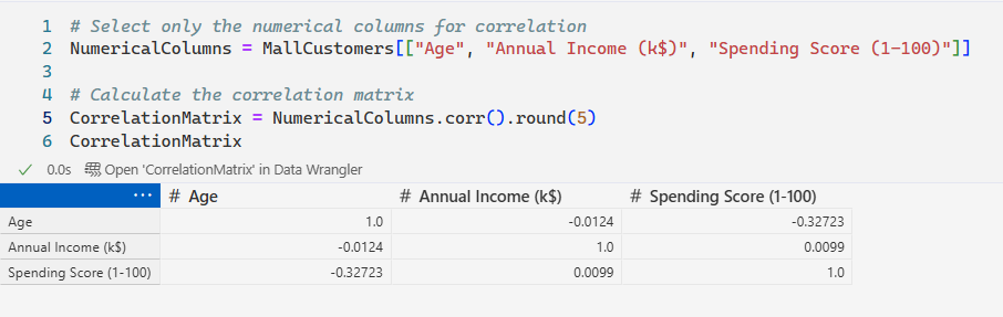
Correlation Matrix of Customer Features

Feature Correlation Matrix Summary
| Relationship | Correlation Coefficient | Interpretation |
|---|---|---|
| Age vs. Spending Score | -0.33 | Weak Negative Correlation. As customers get older, their spending score shows a slight tendency to decrease. |
| Annual Income vs. Spending Score | +0.010 | NO Significant Linear Correlation. The near-zero value confirms that the five distinct clusters seen in the scatter plot are non-linear patterns. |
| Age vs. Annual Income | -0.012 | NO Significant Linear Correlation. Age and income are independent in this dataset. |
Clustering Analysis Summary
This analysis involved three stages of K-Means clustering to robustly segment the mall customers.
- Univariate & Bivariate Segmentation
The initial stages established key market structure:
-
Univariate (Income): Optimal K=3 for high-level income grouping.
-
Bivariate (Income vs. Spending): Optimal K=5, defining the five classic customer segments (e.g., High-Value, Careful, etc.), which is the main marketing deliverable.

|

|
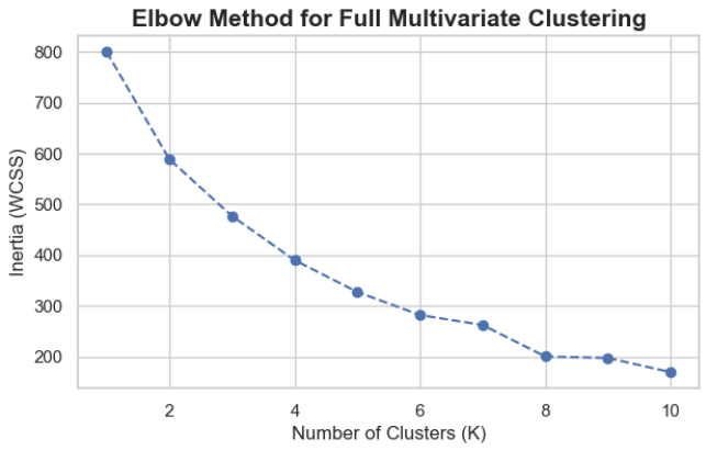
- Multivariate (Full Feature) Segmentation
This stage provides the most actionable and accurate model:
-
Prerequisite: Feature Scaling (StandardScaler) was mandatory to prevent bias from feature range differences.
-
Optimal K (from Elbow Plot): K=4 was determined to be the best-fitting number of segments for the full dataset (Age, Income, Spending, Gender).
-
Final Output: This provides the final, nuanced customer profiles for strategic decision-making.
Final Conclusion: Strategic Value of Customer Segmentation
The analysis confirms the Mall Customers dataset is highly suitable for actionable segmentation, but its value is entirely dependent on Multivariate Analysis, not simple correlation.
Key Analytical Findings
-
Low Predictability: The most critical finding is the near-zero linear correlation between Annual Income and Spending Score ($\approx 0.01$). This proves that income alone is unreliable for predicting a customer’s spending habits.
-
Strategic Segmentation: The analysis successfully defined two optimal segmentation models:
- Bivariate Model (K=5): Ideal for visualizing and communicating the five classic customer types (e.g., High-Value Targets, Careful Spenders). This is the key deliverable for marketing campaign design.
- Multivariate Model (K=4): The final, most statistically robust model. Determined by running K-Means on all scaled features (Age, Income, Spending, Gender), it provides the most comprehensive and nuanced customer profiles for operational decision-making.
Actionable Recommendation
The organization should utilize the $K=4$ or $K=5$ clusters to immediately tailor marketing efforts, product development, and store layout to the specific needs and spending patterns of each identified customer segment.
Author: Maria Egbuna
Project: Mall Customers Segregation Analysis
License: MIT License
Date: September 27, 2025